Quote
as: Pascual-Marqui RD. Reply to Comments Made by R. Grave De Peralta Menendez
and S.I. Gozalez Andino. International Journal of Bioelectromagnetism 1999,
Vol. 1, No. 2, at:
http://www.ee.tut.fi/rgi/ijbem/volume1/number2/html/pascual.htm
Reply to comments made by R. Grave de Peralta Menendez and S.L. Gozalez Andino [10]
Roberto Domingo Pascual-Marqui
![]()
![]()
The
KEY Institute for Brain-Mind Research, University Hospital of Psychiatry, Lenggstr. 31, CH-8029, Zurich,
Switzerland ![]()
c) Quoting from [10], comment “c)”: “The superposition principle cannot be applied to a non linear relationship….”
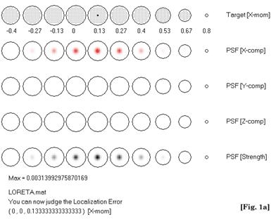
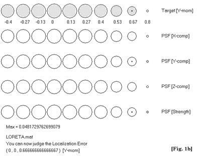
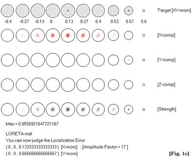
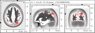
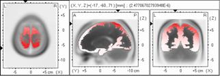
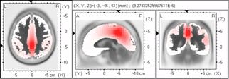
c) My Reply: The principles of linearity and superposition for localization are illustrated in Figure 1. These results (and their generalization) can be replicated by the interested reader, using software that has been available upon request to the author since June 1998 (http://www.keyinst.unizh.ch/loreta.htm). Figures 1a and 1b show LORETA point spread functions for two sources at different depths. The deep source is more blurred than the shallow source. The only way LORETA can resolve both simultaneously active sources is by increasing the strength of the deep source, as shown in Figure 1c (which is the same as Figure 4 in [1]). In general, LORETA can resolve two sources if they are sufficiently separated, and if their estimated strengths are comparable. This is the essence and main property of Low Resolution Brain Electromagnetic Tomography (LORETA): it will always produce a blurred (approximate) image of reality. Blurring will not always allow resolving all maxima. There was never any pompous claim of “high” or “optimum” resolution in LORETA. The main property of LORETA holds.
1.1. Quoting from [10]: “The study of all possible spread functions is equivalent to the analysis of all the resolution kernels [2],[3].”
1.1. My reply: Grave de Peralta Menendez and Gonzalez Andino quote themselves for this statement. They have falsified the truth: this statement is not to be found in their papers [2] and [3]. This statement can be found in my paper [1] (in section “The resolution matrix”). Actually, Grave de Peralta Menendez and Gonzalez Andino have made statements quite to the contrary, scorning the information contained in the point spread functions. For instance, in [2] they state: “The information contained on the impulse responses concerns exclusively single point sources,...” (Note: impulse response and point spread function have the same meaning.)
1.2. Quoting from [10]: “However, the analysis presented by Pascual-Marqui in [1] and [6] to evaluate the solutions is not really using the spread functions but a measure derived from them: The dipole localization error....."
1.2. My reply: In [1] I present an exhaustive analysis of all point spread functions, based on the feature which I consider most relevant to the aim of EEG inverse solutions: localization error. The “dispersion” of point spread functions was defined, studied, and reported in [6]. The computer programs used and offered to the reader in [1] (available upon request to the author since June 1998: http://www.keyinst.unizh.ch/loreta.htm), allow the full and complete exhaustive evaluation of all point spread functions, including amplitudes (see Figure 1).
I define “first order localization errors” of an instantaneous 3D discrete linear inverse solution as the set of localization errors for each point spread function. My methodology for comparing solutions belonging to this class starts with the following two principles: (1) high first order localization errors indicate the inadequacy of a solution; (2) the converse is not true. One essential fact must stressed: while low errors do not indicate adequacy of a solution, they do constitute a necessary (but not sufficient) condition for adequacy of a solution.
2.1. Quoting from [10]: “About the “futility of trying to design near ideal averaging kernels”....”
2.1. My reply: The averaging (or resolution) kernels are harmonic functions. This fact was published in [1], and it proves that in a 3D solution space, the averaging kernels can not be optimized. Therefore, all efforts towards optimization in a 3D solution space, as published and “extensively discussed in the literature ([8], [2], [3])”, have been futile. This fact of nature holds and cannot be changed for a 3D solution space. Any insistence in the rationality of optimization in 3D space is pointless.
I wish to emphasize that the “curse of harmonic resolution kernels” was reported in [1]. It was not reported in the papers by Grave de Peralta Menendez and Gonzalez Andino, a fact that can be confirmed by reading carefully their self-quoted papers. For instance, in [3] they state: “A certain eccentricity value seems to exist below which all solutions fail to obtain adequately centered resolution kernels around the target point.” This statement is a far cry away from the full mathematical characterization implied by the harmonic character of the resolution kernels reported in [1].
One word of caution with respect to the equivalence of resolution kernel and point spread function optimization: Resolution kernels can not be optimized in 3D space, because of their harmonic character. Point spread functions might be amenable to optimization, since, in general, they are not harmonic. However, for optimization to take effect, one must find the proper functional. The WROP functionals in [3] may not necessarily be the best ones. Other functionals for optimizing the full resolution matrix exist, such as the one reported in equation 10, in [1]. This optimization, with the proper weight, produces LORETA, which satisfies “the minimum necessary condition” of low first order localization errors.
2.2. Quoting from [10]: “We are pleased to see that in this paper [1], the author coincides with us….”
2.2. My reply: First, it is worth emphasizing that the definition and interpretation of the averaging kernels for any linear inverse problem were published by Backus and Gilbert [8]. This contribution was not made by Grave de Peralta Menendez and Gonzalez Andino, as they so pretentiously imply. Second, all averaging kernel features emphatically proposed in ([2], [3], [4], [5]) are practically non-informative in 3D space, due to the fact that the averaging kernels are harmonic [1].
3.1. Quoting from [10]: “It is not true that we “omitted an explicit equation of the inverse solution for the case of an unknown vector field”…..”
3.1. My reply: Substitution of the proper weights (given by the unidentified equation following equation 14 in [3]), into equation 14 in [3], is undefined. The authors did not specify in their paper the definition of the product of a Kronecker delta with a lead field. The correct form of equations was originally defined by Backus in Gilbert (see equation (4.10) in [8]), where such a product was specified. The correct explicit equations can also be found in [1].
3.2. Quoting from [10]: “Finally, the author fails to realize that the WROP method is not a particular inverse solution but an strategy…..”
3.2. My reply: Grave de Peralta Menendez et al. proposed the WROP method in [3]. They claimed “optimum resolution”. They did not indicate how to choose the “so-called” weights in WROP. Furthermore, they presented results that are not reproducible by other researchers, since they did not specify the particular weights that were used in creating their Figures. Now the authors claim that the WROP method-strategy is very general. For the researcher interested in testing concrete inverse solutions, the only practical issue is: which WROP weights should be used for realistic (non-spherical) head geometry?
Whatever the case may be, the results in [1] show that the WROP strategy is doomed to failure because in 3D space, optimization is pointless. Moreover, using the WROP strategy with a particular choice of weights [1] was shown to produce an inverse solution incapable of correct first order localization.
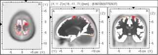
As of this moment, a new software package for the fair comparison of instantaneous 3D discrete linear inverse solutions (for current density) is available upon request to the author (http://www.keyinst.unizh.ch/loreta.htm). This package is based on a somewhat more realistic head model: the average human brain Talairach MRI atlas from McGill University. The approximate EEG lead field was computed numerically using the boundary element method (BEM). No use is made here of “spherical” approximations. Appendix-I includes some new, unambiguously specified, inverse solutions that can be found in the package. Also included here (Appendix-II) is the treatment of the regularization issue. Using a 7 mm resolution grid for the cortical grey matter solution space, the mean localization errors for LORETA and minimum norm were 11.45 and 18.61 mm, respectively. Figure 2 illustrates LORETA and minimum norm images (non-regularized and regularized) due to a point source, in the case of noisy measurements. Regularization was estimated via minimum cross-validation error.
Once Grave de Peralta Menendez and Gonzalez Andino publish a completely specific and unambiguous instantaneous 3D discrete linear inverse solution for current density in non-spherical head models, it will be included in the Talairach package.
3.3. Quoting from [10]: “Then, the conclusion of Pascual-Marqui [1], that “the low localization error, in the sense defined here constitutes a minimum necessary condition” even if apparently reasonable, is not justifiable on theoretical or simulation grounds.”
3.3. My reply: Grave de Peralta Menendez and Gonzalez Andino failed to remember, again, that the principles of linearity and superposition hold (see my reply to comment “c)” above).
3.4. Quoting from [10]: “Earlier conclusions about LORETA (the main properties of LORETA [9]) conjectured on the basis of the dipole localization error have proved to be false.”
3.4. My reply: “Blurring” is certainly equivalent to “distortion”. LORETA produces blurred images (low resolution) of reality (see my reply to comment “c)” above), and therefore, the main properties of LORETA hold.
References
[1] Pascual-Marqui, R.D. “Review of methods for solving the EEG inverse problem”. International Journal of Bioelectromagnetism. No. 1, Vol.1, 1999.
[2] Grave de Peralta Menendez R and Gonzalez Andino SL. “A critical analysis of linear inverse solutions”. IEEE Trans. Biomed. Engn. Vol 4: 440-48. 1998.
[3] Grave de Peralta Menendez R, Hauk O, Gonzalez Andino, S, Vogt H and Michel. CM: “Linear inverse solutions with optimal resolution kernels applied to the electromagnetic tomography.” Human Brain Mapping, Vol 5: 454-67. 1997.
[4] Grave de Peralta Menende R., Gonzalez Andino SL. “Distributed source models: Standard solutions and new developments”. In: Uhl C, ed. Analysis of Neurophysiological Brain Functioning. Heidelberg: Springer Verlag. 1998.
[5] Grave de Peralta Menendez R., Gonzalez Andino SL and Lütkenhönner B. “Figures of merit to compare linear distributed inverse solutions”. Brain Topography. Vol. 9. No. 2:117-124. 1996
[6] Pascual-Marqui, R.D. “Reply to comments by Hämäläinen, Ilmoniemi and Nunez. In ISBET Newsletter No. 6, December 1995. Ed: W. Skrandiws. 16-28.
[7] Grave de Peralta Menendez R, Gonzalez Andino SL, (1998c). Basic limitations of linear inverse solutions: A case study. Proceedings of the 20th annual international conference of the Engineering and Biology Society (EMBS).
[8] Backus G and Gilbert F: The resolving power of gross earth data. Geophys. J. R. Astr. Soc. 16:169-205, 1968.
[9] Pascual Marqui, RD and Michel, CM (1994) LORETA: New Authentic 3D functional images of the brain. In: ISBET Newsletter No. 5, November 1994. Ed: W. Skrandies. 4-8.
[10] Grave de Peralta Menendez R and Gonzalez Andino SL. “Comments on "Review of methods for solving the EEG inverse problem" by R.D. Pascual-Marqui”.
[11] C.R. Rao and S.K. Mitra. Theory and application of constrained inverse of matrices. SIAM J. Appl. Math., 1973, 24: 473-488.
[12] Stone, M. Journal of the Royal Statistical Society, Series B, 1974, 36:111-147.
Introduction
This Appendix extends the results presented in [1]. Here, the following additional instantaneous, 3D, discrete, linear solutions for the EEG inverse problem are considered:
1. Weighted
minimum norm, with weights that normalize (in the ![]() sense) the lead field.
sense) the lead field.
2. LORETA without lead field normalization, with Laplacian having null current density beyond boundary.
3. LORETA without lead field normalization, with singular Laplacian having arbitrary current density beyond boundary.
1. Methods
The reader must refer to [1] for background and notation.
One type of generalized minimum norm inverse problem is:
 (1)
(1)
for any given positive
definite matrix W of dimension
![]() . The solution
is:
. The solution
is:
![]() (2)
(2)
where ![]() denotes the Moore-Penrose
pseudoinverse of
denotes the Moore-Penrose
pseudoinverse of ![]() .
.
1.1. Weighted minimum norm, with weights
that normalize (in the ![]() sense) the lead field
sense) the lead field
In this case:
![]() (3)
(3)
where ![]() is an exponent,
is an exponent,
![]() denotes the Kronecker
product,
denotes the Kronecker
product, ![]() is the identity
is the identity ![]() -matrix, and
-matrix, and ![]() is a diagonal
is a diagonal ![]() -matrix with:
-matrix with:
![]() (4)
(4)
which denotes the ![]() norm, for any
norm, for any ![]() , of the
, of the ![]() vector defined
by:
vector defined
by:
![]() (5)
(5)
Three important comments:
1.
The particular case ![]() corresponds to the classical “minimum
norm”.
corresponds to the classical “minimum
norm”.
2.
The particular case ![]() , p=2
corresponds to the classical “weighted minimum norm”.
, p=2
corresponds to the classical “weighted minimum norm”.
3. This version can be applied to any head geometry, i.e., it is not limited to spherical heads where concepts such as “radius” exist.
1.3. LORETA without lead field normalization, with Laplacian having null current density beyond boundary
In this case:
![]() (6)
(6)
where the matrix B implements a discrete spatial Laplacian
operator. It should be emphasized that such a choice for B produces the smoothest possible inverse
solution. This is because the inverse matrix, i.e. ![]() , implements a discrete spatial smoothing
operator. For a solution space given by a regular cubic 3D grid, with minimum
inter-grid-point distance “d”,
the Laplacian operator used in practice is defined as:
, implements a discrete spatial smoothing
operator. For a solution space given by a regular cubic 3D grid, with minimum
inter-grid-point distance “d”,
the Laplacian operator used in practice is defined as:
 (7)
(7)
Equation (7) corresponds exactly to the Laplacian operator implicitly defined in [6] (see Eq. (2) therein). The explicit definition of the Laplacian is included here (Equation (7)) for the benefit of readers that may be interested in implementing LORETA correctly.
An important comment:
This implements LORETA, without weights, and with boundary condition different from that used previously.
1.4. LORETA without lead field normalization, with singular Laplacian having arbitrary current density beyond boundary
In this case:
![]() (8)
(8)
where the matrix B implements the following discrete spatial Laplacian operator:
 (9)
(9)
Equation (9) corresponds exactly to the Laplacian operator implicitly defined and used in [6] (see Eq. (2’) therein). The explicit definition of the Laplacian is included here (Equation (9)) for the benefit of readers that may be interested in implementing LORETA correctly. The actual boundary condition here is not exactly arbitrary, but rather that the current density at voxels beyond the solution space are certain linear combinations of the nearest neighboring voxels within the solution space.
It should be emphasized that such a choice for B produces the smoothest possible inverse
solution. This is because the pseudo-inverse matrix, i.e.![]() , implements a discrete spatial
smoothing operator. Also, note that B
is singular, with three null eigenvalues, whose corresponding null eigenvectors
are:
, implements a discrete spatial
smoothing operator. Also, note that B
is singular, with three null eigenvalues, whose corresponding null eigenvectors
are:
![]() (10)
(10)
where 1 is an ![]() vector of ones. The null-eigenvectors
correspond to the “spatial DC”.
vector of ones. The null-eigenvectors
correspond to the “spatial DC”.
Because B is singular, the solution given by equation (2) is not valid. The general form of solution for this type of problem can be found in lemma 6.1 in [11]. However, an equivalent simpler derivation will be developed here.
The new problem, which will now be reformulated, can be solved in two steps. In the first step, the problem to be solve is:
![]() (11)
(11)
Note that the minimization
is with respect to J, for some
given C, where C is a 3·1 vector of unknown coefficients, expressing
the contribution of the DC level current density. Note that, by definition
![]() .
.
The solution to the problem expressed in equation (11) is:
![]() (12)
(12)
which depends on C.
The second step consists of solving the problem:
![]() (13)
(13)
which is equivalent to:
![]() (14)
(14)
The solution is:
![]() (15)
(15)
with:
![]() (16)
(16)
Substituting 15 in 12 gives:
 (17)
(17)
Note that ![]() .
.
The total current density estimator is:
![]() (18)
(18)
or equivalently:
 (19)
(19)
An important comment:
This implements LORETA, without weights, and with boundary condition different from that used previously.
Introduction
This Appendix extends the results presented in [1]. Here, regularized instantaneous, 3D, discrete, linear solutions for the EEG inverse problem are considered.
Here I make two propositions. First, ordinary cross-validation is the method of choice for selecting the regularization parameter. Second, in a comparative study of inverse solutions, the method of choice is the inverse solution with minimum cross-validation error. All this work is based on the contributions of Stone [12].
There are two methodological principles involved in judging the performance of an inverse solution:
1. An inverse solution is “not good” if it has high cross-validation error.
2. The converse is not true.
Very informally, the principle states that the selected model must produce the best prediction (in the true sense of objective prediction, as in e.g., the leave-one-out procedure). It is important to emphasize the “prediction error” as defined in the work of Stone [12] is a concept very different from the classical one used in “goodness of fit” and in “least squares”.
1. Methods
The reader must refer to [1] for background and notation.
The regularized version of the generalized minimum norm inverse problem considered is:
![]() (20)
(20)
for any given positive
definite matrix W of dimension
![]() , and for any given
, and for any given
![]() .
This problem and its solution can be found in [6], equations (9), (9’), (10),
(10’) therein.
.
This problem and its solution can be found in [6], equations (9), (9’), (10),
(10’) therein.
Note that K
and ![]() belong
to the linear manifold
belong
to the linear manifold ![]() , where
, where ![]() is the
is the ![]() average reference operator
(or centering matrix) defined as:
average reference operator
(or centering matrix) defined as:
![]() (21)
(21)
where ![]() is an
is an ![]() vector composed
of ones. In this case,
vector composed
of ones. In this case, ![]() ,
, ![]() , and
, and ![]() .
.
The solution to the problem in equation (20) is:
![]() (22)
(22)
The cross-validation error is defined as:
 (23)
(23)
where ![]() denotes the
denotes the ![]() element of
element of ![]() ,
, ![]() denotes the
denotes the ![]() element of the vector
element of the vector ![]() , and:
, and:
![]() (24)
(24)
where ![]() is obtained from
K by deleting its
is obtained from
K by deleting its ![]() row;
row; ![]() ;
; ![]() ;
; ![]() is obtained from
is obtained from
![]() by deleting its
by deleting its ![]() element; and
element; and ![]() .
.
An equivalent equation for cross-validation error is:
 (25)
(25)
where ![]() denotes the eigen-decomposition;
denotes the eigen-decomposition;
![]() is
an
is
an ![]() matrix whose columns
are eigenvectors; and
matrix whose columns
are eigenvectors; and ![]() is an
is an ![]() diagonal matrix with non-null eigenvalues.
diagonal matrix with non-null eigenvalues.
Three important comments:
1. These equations are valid if the matrix W does not depend on the measurement space, i.e., it must not depend on the position or number of electrodes.
2.
Equation (25) is valid for any ![]() .
.
3. I have emphasized here the use of simple ordinary cross-validation as the “common yard stick” for comparing inverse solutions. Ordinary cross-validation corresponds exactly to the concept of “prediction error” based on “leave one out”. Furthermore, it can be calculated exactly for any inverse solution (linear, non-linear, Bayesian, etc.). Generalized cross-validation does not have these properties.
Figures