|
Cite as: “R.D. Pascual-Marqui: Discrete, 3D distributed, linear imaging methods of electric neuronal activity. Part 1: exact, zero
error localization. arXiv:0710.3341 [math-ph], 2007-October-17, http://arxiv.org/pdf/0710.3341 ”
Page 3 of 16
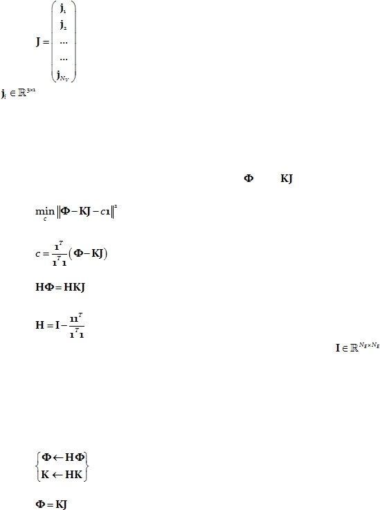
In Eq. 1, J is structured as:
Eq. 8:
where
denotes the current density at the i-th voxel.
3.
The reference electrode problem
As a first step, before even stating the inverse problem, the reference electrode
problem will be solved, by estimating “c” in Eq. 1. Given
and
, the reference electrode
problem is:
Eq. 9:
The solution is:
Eq. 10:
Plugging Eq. 10 into Eq. 1 gives:
Eq. 11:
where:
Eq. 12:
is the average reference operator, also known as the centering matrix, and
is the
identity matrix.
This result establishes the fact that any inverse solution (of any form, not necessarily
linear) will not depend on the reference electrode.
Henceforth, it will be assumed that the EEG measurements and the lead field are
average reference transformed, i.e.:
Eq. 13:
and Eq. 1 will be rewritten as:
Eq. 14:
Note that H
plays the role of the identity matrix for EEG data. It actually is the
identity matrix, except for a null eigenvalue corresponding to an eigenvector of ones (see Eq.
12), accounting for the reference electrode constant.